
The Struggle
Decision-making around Sigma-phase embrittlement is hard. It is not difficult because the mechanism is unknown. API 571 identifies sigma as a hard, brittle Fe–Cr intermetallic whose formation reduces ductility and fracture toughness and can ultimately promote cracking. For AISI 304/304H, the relevant problem is exposure inside a finite thermal window, where chromium diffusion makes nucleation, growth, and coarsening possible. Yet knowing the mechanism is only the beginning for truly applicable decision-making like major maintenance decision. The operational question is not simply whether sigma can form, but how much has formed, how fast that fraction is evolving, and when the resulting loss of material capacity becomes unacceptable from a risk assessment perspective.
That distinction makes sigma unusually difficult to manage compared to other known damage mechanisms:
- Creep assessment seeks a remaining-life quantity;
- Corrosion can often be expressed through wall loss or a corrosion rate;
- Crack-like flaws can be compared with fracture-mechanics acceptance limits.
The sigma problem, in the other hand, doesn't lend itself to easy remaining life calculations. The method propossed in this article try to alleviate such coundrum by twerking with data until we can delivers a metallurgical state variable, the volume fraction (), which modifies the material's capacity to withstand future mechanical and thermal demands. The integrity problem, as approached here, is therefore indirect: first predict the evolving microstructure, then connect that state to degraded properties, then compare degraded capacity with credible demand to finally land in a decision-making outcome.
A big part of the problem with Sigma-Phase is that the risk is "conditional". A sigma-affected component does not fail merely because a precipitate exists. Brittle-fracture susceptibility becomes operationally significant when the degraded material encounters an adverse combination of reduced temperature and significant residual, thermal, pressure, or externally imposed stress. The high-temperature history creates the microstructure; a later demand can "reveal" its consequences. The damage history and the failure-triggering event therefore occupy different parts of the asset’s operating history.
The available evidence is correspondingly difficult to aggregate. Catastrophic sigma-embrittlement failures are infrequent, affected components are often replaced preventively, and each component carries a distinct thermal and microstructural history. Base metal and weld metal cannot be treated as a single statistical population: residual ferrite in welds can accelerate sigma precipitation dramatically compared with fully austenitic base metal. The result is a mechanism of potentially high consequence but scarce and scattered failure data—the exact setting in which a purely empirical failure-frequency model becomes fragile.
Metallurgy can answer how much sigma is present, while conventional risk methods can rank the relative importance of damage, but neither answer alone determines how the risk state evolves continuously with time.
Why API Is Not Enough
API standards remain essential. API 571 defines the mechanism, susceptible materials, temperature ranges, critical factors, inspection considerations, and mitigation logic. API 581 Section 23 provides an RBI procedure for sigma embrittlement and uses estimated sigma content and evaluation temperature to assign damage factors. API 579-1/ASME FFS-1 supplies the broader fitness-for-service language needed to compare demand with degraded capacity. Together, these documents establish the correct "high level" integrity-management architecture.
All above is great, but "devil is in the details". A standards-based framework is not the same as a component-specific forecasting model for decision-making if you have to sing the Go/Hold for the next major maintenance or T/A. API 581 evaluates sigma embrittlement by combining the estimated sigma content with the temperature at which the component is being assessed. Rather than modeling the damage continuously, it places sigma content into three broad categories—Low Sigma (greater than 1% and less than 5%), Medium Sigma (greater than or equal to 5% and less than 10%), and High Sigma (greater than or equal to 10%)—and assigns a corresponding damage factor. This provides a practical and conservative basis for risk screening without requiring a large history of actual sigma-related failures. That conservatism reflects the scarcity and considerable scatter of the available mechanical-property and test data. API 581 therefore assumes, for purposes of calculating the damage factor, that sigmatized austenitic stainless steels behave in a brittle fashion similar to ferritic steels.
API 581 Sigma-Content Screening Categories
| Sigma Content | API 581 Classification |
|---|---|
| >1% and <5% | Low Sigma |
| ≥5% and <10% | Medium Sigma |
| ≥10% | High Sigma |
That method is useful for screening and prioritization, but it leaves several engineering questions unresolved:
- What is the expected sigma fraction at a future operating date?
- How does a real, non-isothermal thermal history move the component toward a metallurgical limit?
- When will an asset-specific threshold be crossed under mean and conservative kinetic scenarios?
- How can measured sigma fraction, rather than only a tabulated category, be carried continuously into reliability calculations?
- How should uncertainty in temperature history, composition, ferrite content, and kinetic parameters alter the timing of inspection or intervention?
The standards do not claim to resolve every such case. API 571 explicitly recognizes that its damage-mechanism descriptions are not definitive instructions for every possible situation. The gap is therefore not a defect in API; it is the natural boundary of a general standard. For sigma phase, the missing layer is a continuous, material-specific connection between precipitation kinetics and decision mathematics.
The proposed JMAK–Weibull framework is designed to occupy that layer. It does not replace API 571, API 581, or API 579-1. It complements them when validated kinetic parameters and metallurgical evidence are available and when greater temporal resolution is required than a discrete screening factor can provide.
From Atoms to a State Variable
Sigma precipitation begins with nucleation. In a metastable austenitic matrix, a cluster of the new phase must overcome an interfacial-energy barrier before it can grow. The classical capillarity description expresses the free energy of a cluster containing atoms as a competition between a favorable volume term and an unfavorable surface term:
The first contribution scales with cluster volume and reflects the thermodynamic driving force; the second scales with interfacial area and penalizes creation of the cluster–matrix interface. Their competition creates a critical cluster size and a nucleation barrier. Subcritical clusters tend to dissolve, whereas supercritical clusters can grow. Chromium diffusion, the steady nucleation rate, the Zeldovich correction, the critical-cluster condensation rate, and the incubation time then govern the microscopic kinetics.
A fully detailed model would track the precipitate population , solve solute-diffusion and population-balance equations, account for continuing nucleation and growth, and integrate the resulting size distribution to obtain the total transformed volume. That route is physically rich but requires thermodynamic, diffusion, interfacial, and initial-microstructure data that are rarely available with sufficient fidelity for an operating component.
The practical alternative is to condense that microscopic machinery into a calibratable macroscopic state equation. The Johnson–Mehl–Avrami–Kolmogorov model does exactly that:
Eq. 1 — JMAK Transformation Law
Here, is the predicted sigma volume fraction, is the maximum attainable fraction for the specific material and temperature, is the effective kinetic constant, and is the Avrami exponent. The parameter condenses nucleation, diffusion-controlled growth, and later coarsening, while reflects the combined influence of nucleation mode and growth dimensionality.
Temperature enters through an Arrhenius-type relation:
Eq. 2 — Arrhenius Temperature Dependence
where is an effective pre-exponential factor, is the effective activation energy, is the universal gas constant, and is absolute temperature. These are not universal constants for "304H" or any other metal. They depend on composition, grain structure, ferrite content, prior thermal and mechanical history, and the specific temperature regime. Calibration is therefore not an accessory to the model; it is part of the model.
Notation at a Glance
| Predicted sigma-phase volume fraction at time t, temperature T | |
| Maximum attainable sigma fraction for the material and temperature | |
| Effective kinetic constant (Arrhenius temperature dependence) | |
| Avrami exponent — nucleation mode and growth dimensionality | |
| Pre-exponential factor, activation energy, gas constant, absolute temperature | |
| Normalized transformed fraction, f_\sigma(t)/f_{\max} | |
| Equivalent Weibull shape and characteristic-time parameters (\beta=n,\ \lambda=k^{-1/n}) | |
| Survival and hazard functions of the equivalent Weibull form | |
| Analyst-calibrated risk-curve shape and characteristic-time parameters | |
| Reference sigma condition’s time and analyst-assigned risk level | |
| Selected metallurgical threshold and its predicted crossing time |
The JMAK–Weibull "Convenient Similarity"
The central insight appears when the metallurgical state variable is normalized:
Eq. 3 — Normalized JMAK Kinetics
For , , and , this function begins at zero, is bounded between zero and one, increases monotonically, and approaches one asymptotically. Those are precisely the mathematical properties required of a cumulative distribution function over non-negative time.
Now compare it with the two-parameter Weibull cumulative distribution:
Eq. 4 — Two-Parameter Weibull CDF
The two equations are not merely similar. They are algebraically identical under the parameter mapping
because . The Avrami exponent becomes the Weibull shape parameter, and the kinetic constant determines the Weibull characteristic time.
This is the mathematical hinge of the methodology. It means that a sigma-transformation curve calibrated from metallurgical evidence can be written in the same formal language used to construct reliability metrics. The corresponding survival-form function is
and the associated hazard-form function is
which is exactly the standard Weibull hazard with and . The mapping therefore extends beyond the cumulative curve: it carries the transformation kinetics into characteristic time, survival, hazard, and percentile calculations without changing the underlying parameter set.
The "discovery" is not simply that two equations look alike; that formal analogy has precedent in the literature summarized in the project documentation. The contribution is to operationalize the equivalence for sigma-phase integrity management: use JMAK to preserve the physics of nucleation and growth, use the Weibull representation to obtain a continuous time-based decision language, and then reconnect that language to explicit metallurgical and mechanical acceptance criteria.
The equivalent Weibull function defined in this section is not yet the owner-calibrated risk curve used for decision-making. It is an exact mathematical restatement of normalized JMAK kinetics and therefore coincides with the JMAK trajectory. The decision model introduced later uses the time at which JMAK reaches a selected reference sigma condition, but it allows the analyst to assign the risk associated with that condition. That additional risk-appetite calibration produces separate parameters and ; consequently, the resulting risk curve need not coincide with the equivalent Weibull-form transformation curve.
Central Warning: Mathematical Equivalence Is Not Physical Identity
The framework must preserve one critical distinction. The normalized transformed fraction is a metallurgical quantity. A Weibull cumulative probability is a probabilistic reliability quantity. Their equality of form does not prove that "4% sigma" is a 4% probability of failure, nor does it prove that precipitation alone determines component failure.
A defensible interpretation requires a causal chain:
Sigma-phase fraction predicted by JMAK kinetics
Reduced toughness, ductility, or another governing property
Lower load- or damage-bearing capability of the component
Comparison of credible operating demand against remaining capacity
Point at which the governing acceptance limit is exceeded
That chain requires material-specific evidence connecting sigma fraction and morphology to effective toughness, ductility, or another property relevant to the governing failure mode. It also requires a defined mechanical-demand model. Without those links, the Weibull-form result is a risk indicator derived from kinetics, not a validated probability of component failure.
Critical Caveat
This limitation strengthens rather than weakens the method. It prevents an algebraic correspondence from being promoted into an unsupported physical claim. The framework becomes a disciplined translation layer: mathematically exact in its parameter mapping, physically conditional in its interpretation, and explicitly dependent on calibration and validation.
From a Curve to Decisions
The value of a continuous model becomes evident when an engineering limit is introduced. Let denote a selected metallurgical threshold, defined for the relevant material, location, microstructure, and demand scenario. Solving the JMAK equation for the time at which this threshold is reached gives
Eq. 5 — Threshold-Crossing Time (Decision Equation)
This equation converts an acceptance criterion into a forecast date. It does not, by itself, declare failure. It identifies when the predicted metallurgical state reaches a boundary beyond which original catalog properties should no longer be assumed without recaracterization.
The project methodology distinguishes an early operational change-of-regime threshold from a more severely embrittled state. For 304/304H, the conservative trajectory approaching roughly 1% sigma is treated as a trigger for directed confirmation and reassessment, especially in welds or ferrite-bearing regions; fractions in the 3–5% range are treated as clearly embrittled conditions requiring explicit consideration of degraded toughness and brittle-fracture susceptibility. These are operational criteria within the developed framework, not universal material constants, and they must be challenged against the stability of mechanical demand, cooling events, microstructure, and the quality of the underlying measurements.
This is where risk appetite enters the framework without altering the metallurgical model. JMAK predicts the evolution of sigma phase and determines the time at which a selected reference sigma condition is reached. The analyst then assigns the level of risk that the asset owner is prepared to associate with that reference condition, considering the consequence of failure, operating context, inspection capability, and organizational risk appetite. That time-risk anchor, together with the selected Weibull shape parameter, calibrates the Weibull risk curve. Consequently, the JMAK transformation curve and the Weibull risk curve are not required to coincide: they represent different quantities and may produce different values at the same exposure time. The JMAK curve represents predicted metallurgical progression, whereas the Weibull curve represents the risk assigned to that progression through the analyst-defined calibration. The formal JMAK–Weibull similarity provides the mathematical bridge; the risk-appetite calibration determines the position of the risk curve.
Real Thermal Histories
Plant equipment rarely experiences a perfectly isothermal exposure. Applying JMAK kinetics to a variable-temperature history therefore requires more than independently adding the transformation produced in each thermal block. The metallurgical state accumulated before a new block must first be converted into an equivalent isothermal age at the temperature of that block.
For a calibrated temperature interval in which and can reasonably be treated as constant, define the normalized sigma fraction at the beginning of block as
The previous metallurgical state is converted into an equivalent exposure time at the new block temperature :
After exposure for at , the normalized transformed fraction becomes
and the absolute sigma fraction is
This equivalent-time procedure preserves the previously accumulated metallurgical state while evaluating subsequent transformation at the kinetics applicable to the new temperature. It also ensures that subdividing an isothermal interval into smaller blocks does not, by itself, change the predicted sigma fraction.
The formulation is applicable only within the range over which , , and have been calibrated and the governing precipitation mechanism remains unchanged. If , , or the active transformation mechanism changes significantly with temperature, the history must be divided into separately calibrated regimes with validated transition rules; the simple equivalent-time construction must not be extrapolated across those regimes.
Exposure below the active sigma-formation range may be treated as kinetically inactive while retaining the sigma fraction already formed, because cooling suppresses diffusion without automatically restoring the original austenitic microstructure. Excursions above the applicable sigma-stability range require separate consideration of dissolution kinetics and must not automatically be treated as inactive exposure with perfect retention.
The operating record may be divided into approximately isothermal blocks, but the selected temperature-deviation criterion is a numerical implementation parameter rather than a universal metallurgical constant. Its adequacy must be demonstrated through a time-step and block-size sensitivity study. The predicted history is acceptable only when further refinement of the thermal segmentation produces no material change in the sigma-fraction trajectory or threshold-crossing time.
The Algorithmic Instrument
The methodology can be implemented as a structured engineering workflow that converts operating history and metallurgical evidence into an integrity decision:
The confidence placed in the result must match the quality of the parameters. Level 3 data can support equipment prioritization and identify where targeted measurements are needed, but they are not sufficient for high-consequence decisions such as extending service life or deferring replacement. Those decisions require Level 2 or, preferably, Level 1 calibration. In every case, the conservative uncertainty boundary—not a single deterministic prediction—must govern the timing of action.
What the Framework Adds
The framework adds resolution where API screening is necessarily discrete. It supplies a continuous forecast of sigma evolution, preserves the distinction between base and weld kinetics, accepts real thermal histories, exposes parameter uncertainty, and calculates when a selected state or risk boundary will be reached. It can therefore inform inspection timing before a tabulated damage category changes.
It also creates a mathematically coherent interface between two engineering disciplines. Metallurgy retains ownership of , , , microstructure, and the physical meaning of . Reliability engineering gains access to the Weibull parameters and , the survival function , the hazard function , and percentile times. Fitness-for-service analysis then closes the chain by comparing demand with capacity calculated from appropriately degraded properties.
Most importantly, the framework remains subordinate to evidence. It requires validation with field or laboratory data, component-specific calibration, and verification against documented metallurgical observations. It evaluates sigma embrittlement as one mechanism and does not eliminate the need to assess creep, corrosion, thermal fatigue, cracking, or other interacting damage mechanisms under API 571 and API 581.
Example: Turning Metallurgy into an Operating Decision
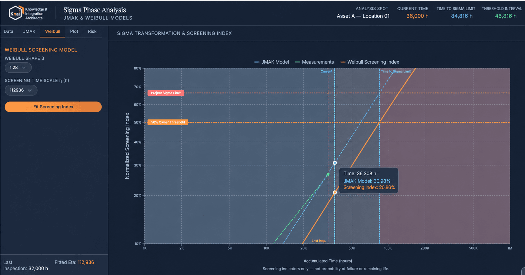
Decision dashboard: JMAK forecast, equivalent Weibull screening index, and measurement curve plotted against accumulated exposure time, with the current-time marker, time-to-sigma-limit marker, and threshold interval called out. As the chart's own footer notes, these are screening indicators only — not a probability of failure or remaining life.
The figure shows how the methodology converts a small set of metallurgical observations into a forward-looking integrity assessment.
Interpretation Note
The JMAK and Weibull risk curves are not expected to coincide. JMAK predicts normalized sigma-phase transformation; the Weibull curve represents risk calibrated by the analyst against a selected reference sigma condition. The risk curve is a screening and decision-support construct unless validated against component failure or performance data.
Inspection measurements are plotted against accumulated exposure time and used to calibrate the JMAK curve, which describes the expected progression of sigma-phase precipitation. The corresponding Weibull representation translates that kinetic trajectory into familiar reliability metrics—characteristic time, percentiles, and threshold-crossing dates—while preserving the distinction between transformed material fraction and probability of failure.
Worked Example — Key Figures
| Current operating exposure | 30,000 hours |
| Projected threshold crossing | ~100,000 hours |
| Nominal planning interval | 70,000 hours |
At 30,000 operating hours, the component remains below the selected intervention limit. Based on the fitted kinetics, that limit is projected to be reached at approximately 100,000 hours, leaving a nominal planning interval of 70,000 hours. This is not a declaration of safe remaining life. It is the estimated time to a defined metallurgical decision point, conditional on the assumed operating history, the validity of the calibrated parameters, and the absence of material changes or more severe thermal exposure.
The dashboard is intended to make that distinction operationally useful. Inspection data establish the observed condition; the JMAK model projects the evolution of sigma phase; and the Weibull form provides a practical time scale for inspection, fitness-for-service assessment, operating controls, and replacement planning. The horizontal criteria allow metallurgical and owner-defined limits to be assessed simultaneously, while the vertical markers connect those limits to the equipment's operating timeline.
The resulting forecast must be interpreted with its uncertainty, not as a single deterministic date. If parameter quality or thermal-history reconstruction is weak, the figure is appropriate for screening and inspection prioritization. Decisions involving life extension, replacement deferral, or demanding future transients require stronger calibration and must be based on the conservative boundary of the prediction range.
Conclusion
The main value of this methodology is that it transforms sigma-phase evaluation from a purely metallurgical observation into a decision-support instrument. Instead of stopping at the statement that a material contains a given fraction of sigma phase, the method connects that technical measurement with a time-dependent representation of risk, making it possible to discuss degradation in a language that supports inspection, operation, maintenance, and replacement decisions.
Its contribution is not limited to estimating sigma fraction. By exploiting the exact formal equivalence between normalized JMAK kinetics and the Weibull cumulative distribution, the methodology creates a forecasting framework that explains how the metallurgical state progresses as thermal exposure accumulates. The same parameter set can then generate characteristic time, survival-form, hazard-form, and threshold-crossing metrics—while preserving the essential distinction between transformed fraction and physical probability of failure.
A second key value is that the method creates a bridge between measurement and management. Sigma fraction remains the technical anchor, but it can be interpreted together with a maximum allowable metallurgical state, degraded mechanical properties, credible operating demand, uncertainty, and organizational risk appetite. The result is not a replacement for API 571, API 581, or API 579-1; it is the missing continuous layer between their damage-mechanism, RBI, and fitness-for-service functions.
Metallurgical evidence, kinetic modeling, reliability mathematics, and integrity criteria converge into one interpretable algorithm. The output is not an automatic life verdict and not a substitute for engineering judgment. It is a stronger mathematical basis for that judgment.